Announcing ggforce: Accelerating ggplot2

I am very pleased to announce the first release of the ggforce package. ggforce is a general ggplot2 extension package in the same vein as ggalt with no overarching goal other than to provide additional functionality to the ggplot2 universe. The inception and birth of ggforce was documented in a recent post and the road to CRAN has been long and winding, with my personal goal of the package going through multiple iterations. At the beginning it was meant as a place where everyone could submit extensions to. As I began working on ggraph it became a dumping ground for functionality that was broader than network visualization, and as I began working on ggplot2 it became a testing ground for new facetting functions. Now, as it is ready for CRAN, it does include some requests and code from other developers, thus paying partial homage to the founding goal of the package.

This post will not go into detail with every functionality that ggforce adds to ggplot2. ggforce includes a vignette where every feature is described along with motivation and code examples.

Features

Below follows a description of all the major features (small utility functions are not included), grouped by the grammar they extend:

Geoms

• geom_arc() allows you to plot circle segments defined by center, radius, and start- and end-angle.
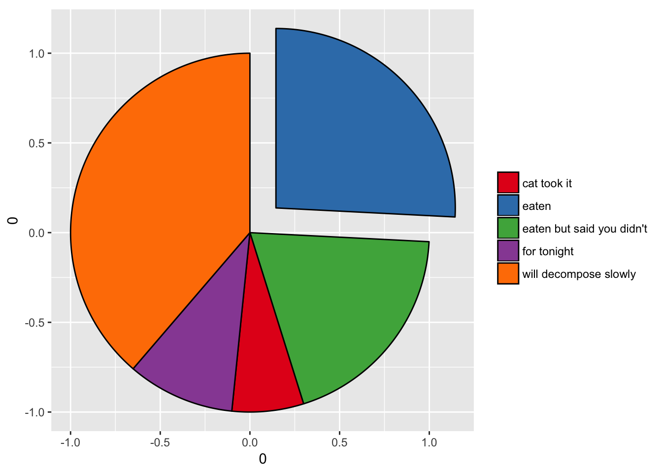
• geom_arc_bar() is as above, except it draws a thick arc defined by an inner and outer radius. If the inner radius is zero it becomes a wedge.

pie <- data.frame(
    state = c('eaten', 'eaten but said you didn\'t', 'cat took it', 
              'for tonight', 'will decompose slowly'),
    focus = c(0.2, 0, 0, 0, 0),
    start = c(0, 1, 2, 3, 4),
    end = c(1, 2, 3, 4, 2*pi),
    amount = c(4,3, 1, 1.5, 6),
    stringsAsFactors = FALSE
)
ggplot(pie) + 
    geom_arc_bar(aes(x0 = 0, y0 = 0, r0 = 0, r = 1, amount = amount, 
                     fill = state, explode = focus), stat = 'pie') + 
    scale_fill_brewer('', palette = 'Set1') +
    coord_fixed()

• geom_circle() makes it possible to draw circles based on coordinate space, that is, the radius is scaled to the coordinate system rather than absolute.
• geom_link() is like geom_segment() except it expands the line into multiple segments making it possible to draw gradients over the line.
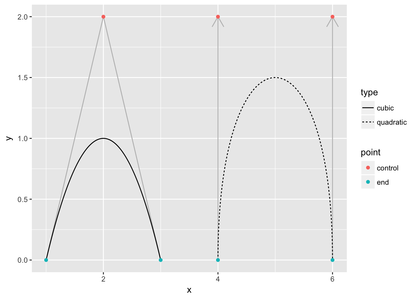
• geom_bezier() allows you to draw cubic and quadratic beziers.

beziers <- data.frame(
    x = c(1, 2, 3, 4, 4, 6, 6),
    y = c(0, 2, 0, 0, 2, 2, 0),
    type = rep(c('cubic', 'quadratic'), c(3, 4)),
    point = c('end', 'control', 'end', 'end', 'control', 'control', 'end')
)
help_lines <- data.frame(
    x = c(1, 3, 4, 6),
    xend = c(2, 2, 4, 6),
    y = 0,
    yend = 2
)
ggplot() + geom_segment(aes(x = x, xend = xend, y = y, yend = yend), 
                        data = help_lines, 
                        arrow = arrow(length = unit(c(0, 0, 0.5, 0.5), 'cm')), 
                        colour = 'grey') + 
    geom_bezier(aes(x= x, y = y, group = type, linetype = type), 
                data = beziers) + 
    geom_point(aes(x = x, y = y, colour = point), data = beziers)

• geom_bspline() makes it possible to draw b-splines.
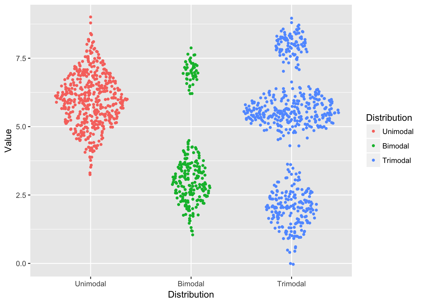
• geom_sina() is a novel alternative to geom_violin()/geom_boxplot()/geom_jitter() that was submitted to ggforce by the developers of sinaplot

df <- data.frame(
  "Distribution" = factor(c(rep("Unimodal", 500),
                     rep("Bimodal", 250),
                     rep("Trimodal", 600)), c('Unimodal', 'Bimodal', 'Trimodal')),
  "Value" = c(rnorm(500, 6, 1),
              rnorm(200, 3, .7), rnorm(50, 7, 0.4),
              rnorm(200, 2, 0.7), rnorm(300, 5.5, 0.4), rnorm(100, 8, 0.4))
)
ggplot(df, aes(Distribution, Value)) + 
    geom_sina(aes(colour = Distribution), size = 1)

Scales

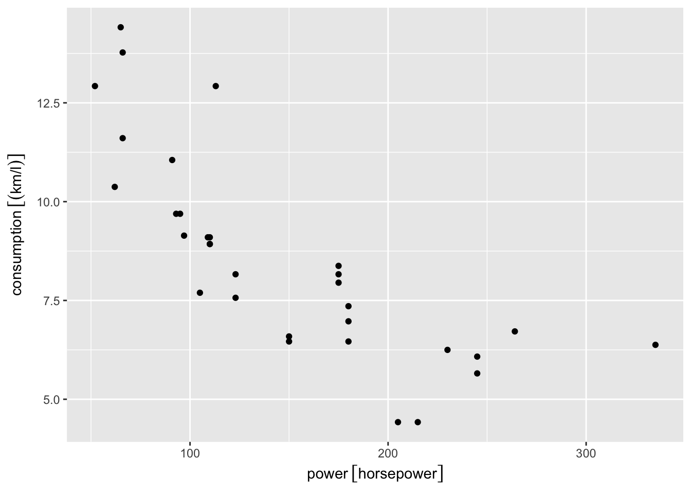
• scale_[x|y]_unit() provides support for the units class from the units package. It provides automatical labelling of axis with units as well as changing the units of the scale without touching the data.

library(units)
miles <- make_unit('miles')
gallon <- make_unit('gallon')
horsepower <- make_unit('horsepower')
mtcars$consumption <- mtcars$mpg * (miles/gallon)
mtcars$power <- mtcars$hp * horsepower

ggplot(mtcars) +
    geom_point(aes(power, consumption)) +
    scale_y_unit(unit = 'km/l')

Facets

• facet_[grid|wrap]_paginate() allows you to split grid and wrap facetting out into multiple pages.
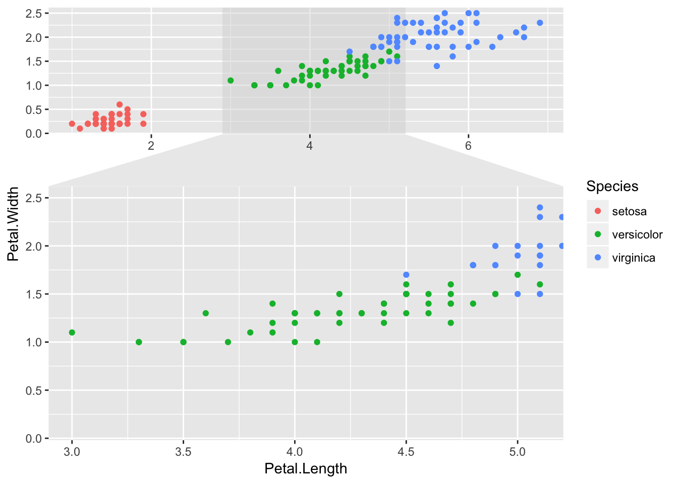
• facet_zoom() is a third zooming alternative that provides a context overview.

ggplot(iris, aes(Petal.Length, Petal.Width, colour = Species)) +
    geom_point() +
    facet_zoom(x = Species == "versicolor")

Transformations

While transformations are part of the scales package rather than ggplot2 their use is integral to ggplot2, and ggforce thus fills some gaps in this department as well.

• power_trans() lets you create any power transformation (scales only provides sqrt_trans()).
• radial_trans() lets you translate between coordinates specified by radius and angle and coordinates specified by x and y.
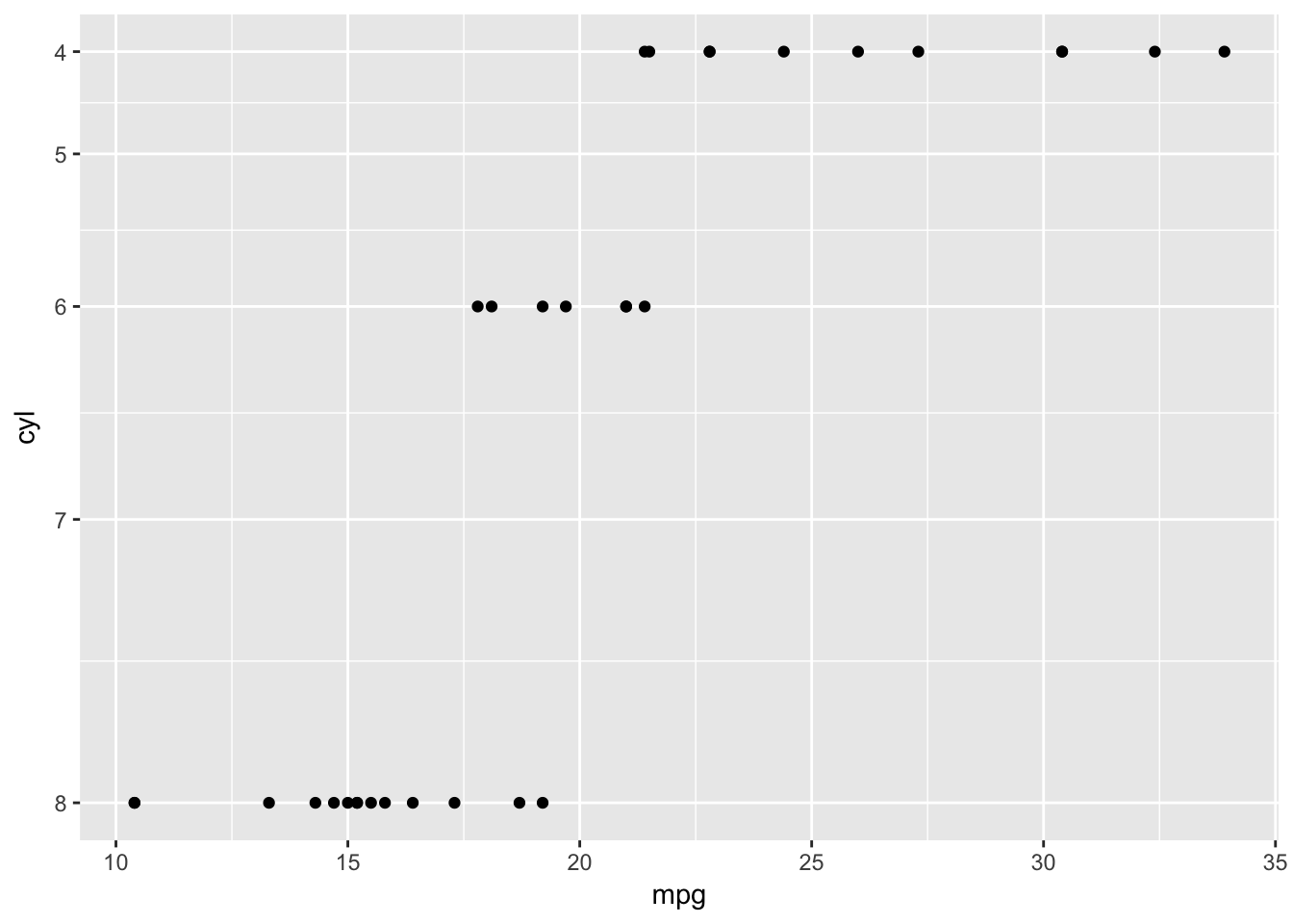
• trans_reverser() reverses any monotonous transformation function, making it possible to e.g. have a reversed log transformation (scales only provides reverse_trans() for reversing the identity transformation).

p3 <- power_trans(3)
p3r <- trans_reverser(p3)
ggplot(mtcars) + 
    geom_point(aes(mpg, cyl)) + 
    scale_y_continuous(trans = p3r)

Future

I have many cool ideas planned for future releases, and I hope that users will approach me if they have some great ideas as well. If you have a burning wish for something in the ggplot2 ecosystem I welcome any issues and PRs on the ggforce github repository. The ggplot2 ecosystem is thriving though so please visit http://www.ggplot2-exts.org and see if your idea doesn’t already exist in another package.

Happy plotting!