I made a 3D movie with ggplot2 once - here’s how I did it
Some time ago (last year actually 😳) I had a blast developing a feature for ggforce which had been on my mind for far to long than its limited utility warranted. The idea was to showcase the new facetting extension powers I’d added to ggplot2 by making a facetting function that created a stereoscopic pair of plots that would simulate 3D. To procrastinate and show off I made a little animated video with the feature and posted it on Twitter, promising I’d write about it someday. Now (again, one year later), I think the world is finally ready to see what went through my R console to make that little animation. While I’ve been very timely with this blog post, the feature is still not available on CRAN, so you’ll need to install the GitHub version of ggforce to follow along.
devtools::install_github('thomasp85/ggforce')Setup
The goal is to create a spinning hollow cube so we’ll need to define the cube somehow. This was way before ggraph was published, and tidygraph was not even a thought in my head, so while it may make sense to handle the cube as a network, I did it the hard way:
library(ggplot2)
library(ggforce)

# Define the corners of the cube
cube <- matrix(
  c(
     1,  1,  1,
     1, -1,  1,
    -1, -1,  1,
    -1,  1,  1,
     1,  1, -1,
     1, -1, -1,
    -1, -1, -1,
    -1,  1, -1
  ),
  ncol = 3, byrow = TRUE
)

# Define each edge - practically making a network the hard way
segments <- data.frame(
  ind = c(1, 2,
          2, 3,
          3, 4,
          4, 1,
          5, 6,
          6, 7,
          7, 8,
          8, 5,
          1, 5,
          2, 6,
          3, 7,
          4, 8),
  group = rep(1:12, each = 2)
)
Now that we have our data, we need to create some transformation functions. Currently, if plotted in ggplot2 it would just look like a square as, unsurprisingly, the third dimension would get lost. What we need is a projection of three dimension down to two. This is a bit hairy, and when I tried to achieve this back in the days by setting up a transformation matrix manually I failed miserably (if you are knowledgable in this and want to explain it to me - please reach out on twitter). In the end I took the shortcut and used the persp() function, which, besides the side effect of plotting stuff in 3D, also returns the transformation matrix invisibly:
tr_mat <- persp(z = cube, theta = 0, phi = 0,
                xlim = c(-2, 2), ylim = c(-2, 2), zlim = c(-2,2))
Having a look at the transformation matrix I can safely say that I have no idea what’s going on:
tr_mat
#>      [,1]         [,2]          [,3]          [,4]
#> [1,]  0.5 0.000000e+00  0.000000e+00  0.000000e+00
#> [2,]  0.0 3.061617e-17 -5.000000e-01  5.000000e-01
#> [3,]  0.0 5.000000e-01  3.061617e-17 -3.061617e-17
#> [4,]  0.0 0.000000e+00 -2.732051e+00  3.732051e+00
But that doesn’t matter - the only thing required is that I know how to use it. The trans3d() provides the means for taking in three dimensional points, and a transformation matrix, and outputting two dimensional points:
trans_cube <- trans3d(cube[,1], cube[,2], cube[,3], tr_mat)
ggplot(as.data.frame(trans_cube)) +
  geom_point(aes(x, y))
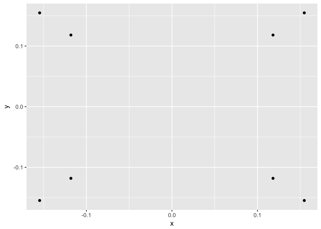
With a bit of imagination we can see the 3D cube. Lets draw it with line segments as well - we add the added information of depth, which is simply the value in the dimension that gets dropped in the transformation.
to_grid <- function(mat, segments, tr_mat) {
  trans <- trans3d(mat[, 1], mat[, 2], mat[, 3], tr_mat)
  cube <- cbind(as.data.frame(trans), depth = -mat[, 2])
  cbind(cube[segments$ind, ], segments)
}
cube_grid <- to_grid(cube, segments, tr_mat)

ggplot(cube_grid) +
  geom_path(aes(x, y, group = group))
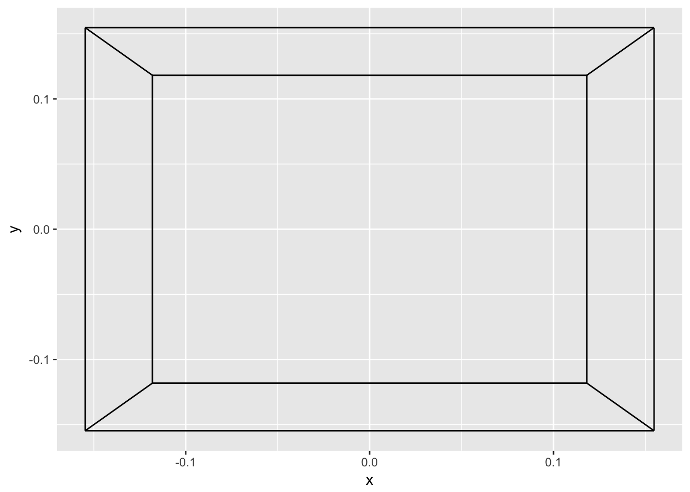
We can of course improve the illusion even more. Using geom_link2() from ggforce, we can add a gradient size to the lines, based on the depth of the endpoints (remember, these were added in the to_grid() function).
ggplot(cube_grid) +
  geom_link2(aes(x, y, group = group, size = depth), lineend = 'round', n = 500) +
  scale_size(range = c(1.5, 3))
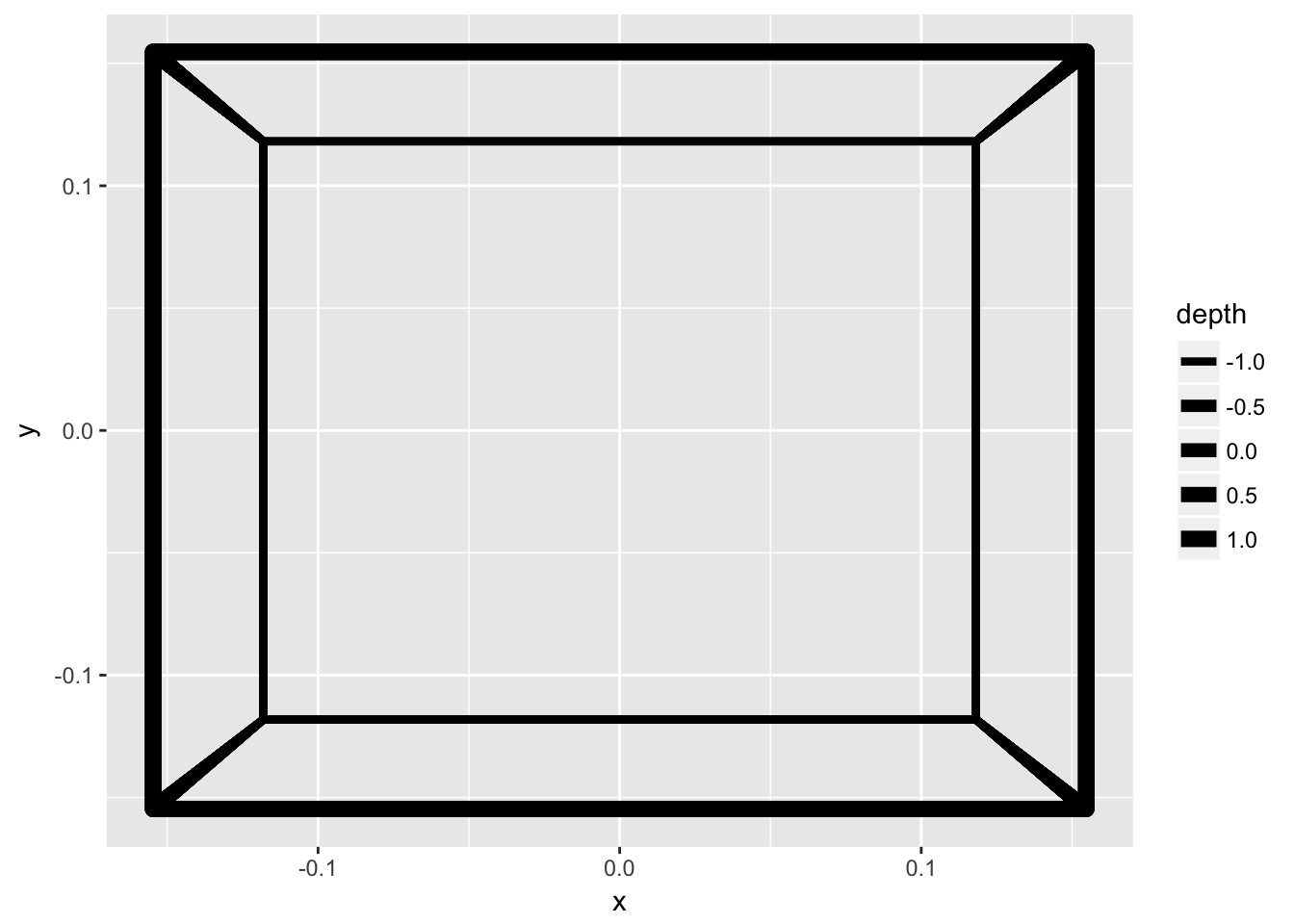
What can we do more? Well, we could decide to rotate it a bit. Let’s, make a function that rotates it around the vertical axis:
rot <- function(mat, angle) {
  mat_tmp <- mat
  mat_tmp[,1] <- mat[,1] * cos(angle) - mat[,2] * sin(angle)
  mat_tmp[,2] <- mat[,2] * cos(angle) + mat[,1] * sin(angle)
  mat_tmp
}

cube_grid <- to_grid(rot(cube, pi/4.5), segments, tr_mat)
ggplot(cube_grid) +
  geom_link2(aes(x, y, group = group, size = depth), lineend = 'round', n = 500) +
  scale_size(range = c(1.5, 3))
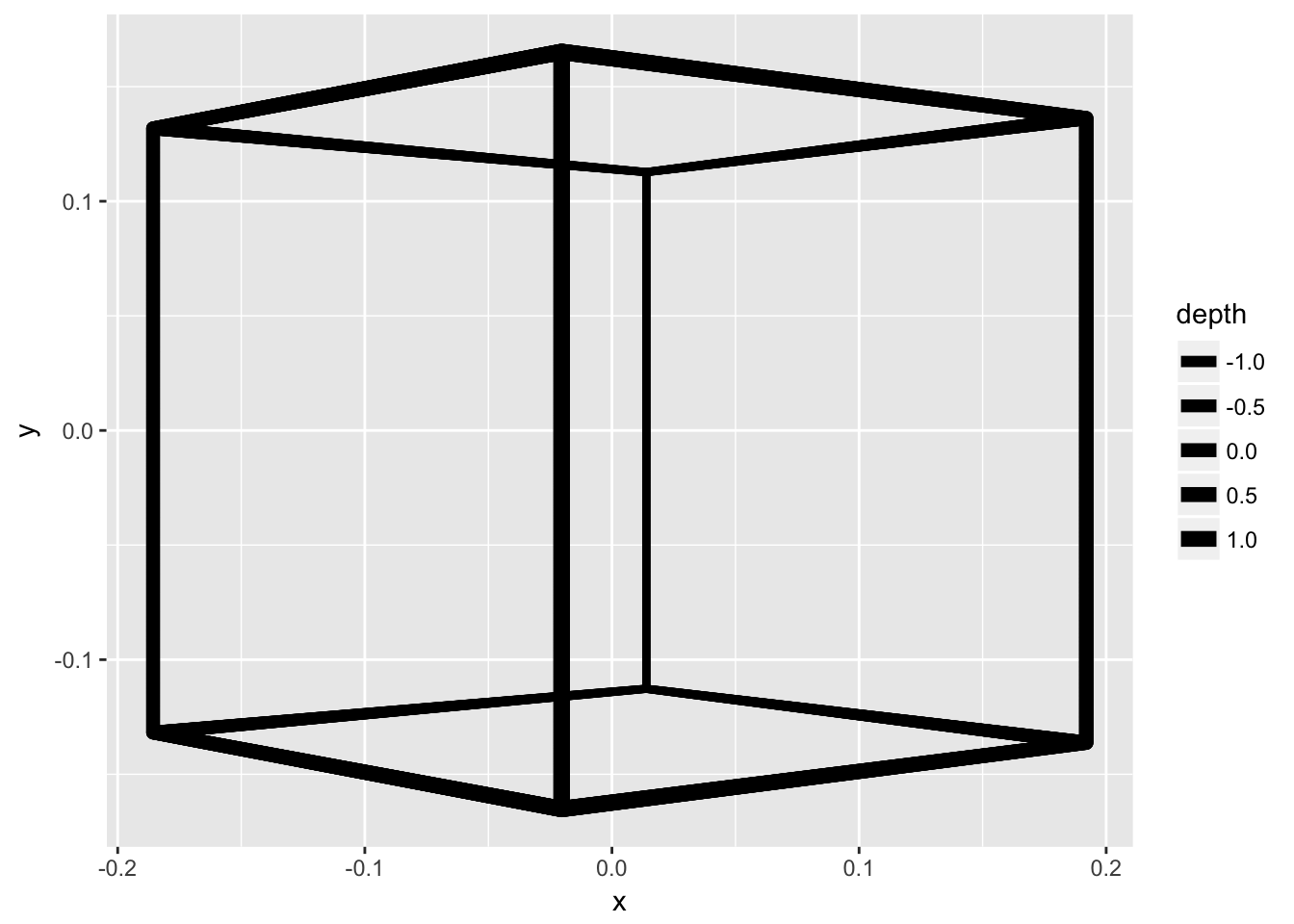
We now have all the ingredients to make an animation of a spinning cube - we really only need to animate a 90 degree spin as it is selfrepeating. For added fiz we’ll improve the depth perception by simulating a bit of haze by greying parts more distant:
angles <- head(seq(0, pi/2, length.out = 51), 50)
cubes <- lapply(angles, function(i) to_grid(rot(cube, i), segments, tr_mat))

for (d in cubes) {
  p <- ggplot(d) +
    geom_link2(aes(x, y, group = group, size = depth, color = depth),
               lineend = 'round', n = 500) +
    scale_size(range = c(1.5, 3)) +
    scale_color_gradient(low = 'grey70', high = 'black') +
    scale_x_continuous(limits = c(-0.4, 0.4)) +
    scale_y_continuous(limits = c(-0.4, 0.4)) +
    coord_fixed() +
    theme(legend.position = 'none')
  plot(p)
}
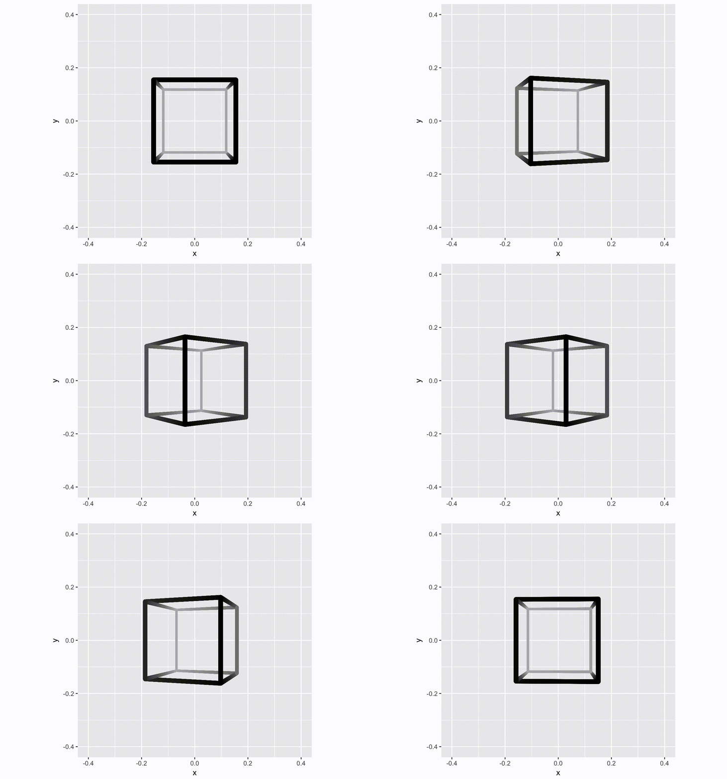
That’s all fine and well, but this is just a regular and boring 2D video. Let us update it to the brave new world, where Avatar has taught us that 3D is not tacky: Enter facet_stereo().
for (d in cubes) {
  p <- ggplot(d) +
    geom_link2(aes(x, y, group = group, size = depth, color = depth,
                   depth = depth), # This tells facet_stereo about depth
               lineend = 'round', n = 500) +
    scale_size(range = c(1.5, 3)) +
    scale_color_gradient(low = 'grey70', high = 'black') +
    scale_x_continuous(limits = c(-0.4, 0.4)) +
    scale_y_continuous(limits = c(-0.4, 0.4)) +
    coord_fixed() +
    theme(legend.position = 'none') +
    scale_depth(range = c(0, 0.15)) + # This scales depth perception
    facet_stereo(panel.size = 200) # This calculates the stereoscopic distortion
  plot(p)
}
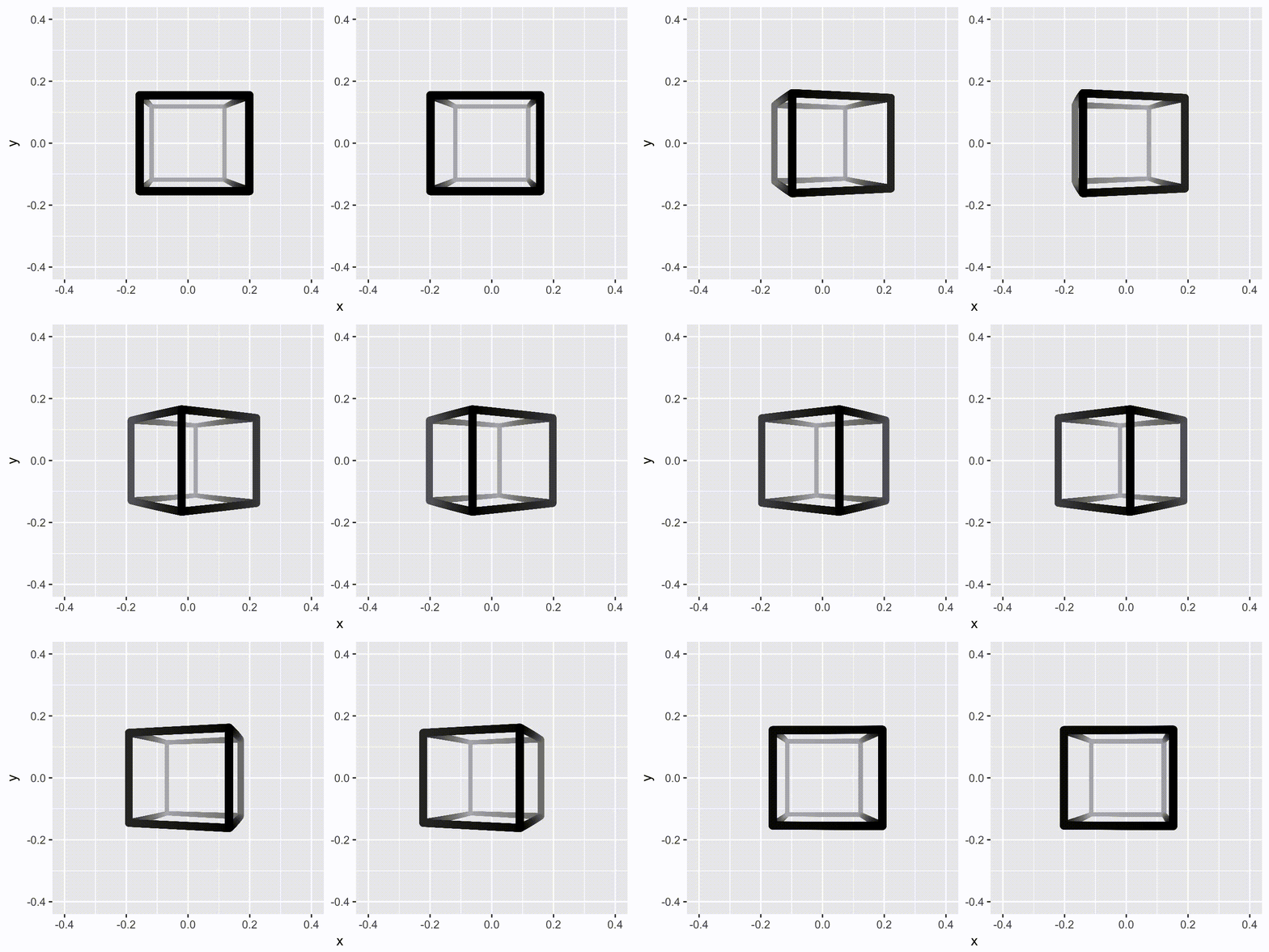
That is all it takes…