lime v0.4: The kitten picture edition

announcement

lime

machine learning

prediction

modelling

March 6, 2018

I’m happy to report a new major release of lime has landed on CRAN. lime is an R port of the Python library of the same name by Marco Ribeiro that allows the user to pry open black box machine learning models and explain their outcomes on a per-observation basis. It works by modelling the outcome of the black box in the local neighborhood around the observation to explain and using this local model to explain why (not how) the black box did what it did. For more information about the theory of lime I will direct you to the article introducing the methodology.

New features

The meat of this release centers around two new features that are somewhat linked: Native support for keras models and support for explaining image models.

keras and images

J.J. Allaire was kind enough to namedrop lime during his keynote introduction of the tensorflow and keras packages and I felt compelled to support them natively. As keras is by far the most popular way to interface with tensorflow it is first in line for build-in support. The addition of keras means that lime now directly supports models from the following packages:

If you’re working on something too obscure or cutting edge to not be able to use these packages it is still possible to make your model lime compliant by providing predict_model() and model_type() methods for it.

keras models are used just like any other model, by passing it into the lime() function along with the training data in order to create an explainer object. Because we’re soon going to talk about image models, we’ll be using one of the pre-trained ImageNet models that is available from keras itself:

library(keras)
library(lime)
library(magick)

model <- application_vgg16(
  weights = "imagenet",
  include_top = TRUE
)
model

## Model
## ___________________________________________________________________________
## Layer (type)                     Output Shape                  Param #     
## ===========================================================================
## input_1 (InputLayer)             (None, 224, 224, 3)           0           
## ___________________________________________________________________________
## block1_conv1 (Conv2D)            (None, 224, 224, 64)          1792        
## ___________________________________________________________________________
## block1_conv2 (Conv2D)            (None, 224, 224, 64)          36928       
## ___________________________________________________________________________
## block1_pool (MaxPooling2D)       (None, 112, 112, 64)          0           
## ___________________________________________________________________________
## block2_conv1 (Conv2D)            (None, 112, 112, 128)         73856       
## ___________________________________________________________________________
## block2_conv2 (Conv2D)            (None, 112, 112, 128)         147584      
## ___________________________________________________________________________
## block2_pool (MaxPooling2D)       (None, 56, 56, 128)           0           
## ___________________________________________________________________________
## block3_conv1 (Conv2D)            (None, 56, 56, 256)           295168      
## ___________________________________________________________________________
## block3_conv2 (Conv2D)            (None, 56, 56, 256)           590080      
## ___________________________________________________________________________
## block3_conv3 (Conv2D)            (None, 56, 56, 256)           590080      
## ___________________________________________________________________________
## block3_pool (MaxPooling2D)       (None, 28, 28, 256)           0           
## ___________________________________________________________________________
## block4_conv1 (Conv2D)            (None, 28, 28, 512)           1180160     
## ___________________________________________________________________________
## block4_conv2 (Conv2D)            (None, 28, 28, 512)           2359808     
## ___________________________________________________________________________
## block4_conv3 (Conv2D)            (None, 28, 28, 512)           2359808     
## ___________________________________________________________________________
## block4_pool (MaxPooling2D)       (None, 14, 14, 512)           0           
## ___________________________________________________________________________
## block5_conv1 (Conv2D)            (None, 14, 14, 512)           2359808     
## ___________________________________________________________________________
## block5_conv2 (Conv2D)            (None, 14, 14, 512)           2359808     
## ___________________________________________________________________________
## block5_conv3 (Conv2D)            (None, 14, 14, 512)           2359808     
## ___________________________________________________________________________
## block5_pool (MaxPooling2D)       (None, 7, 7, 512)             0           
## ___________________________________________________________________________
## flatten (Flatten)                (None, 25088)                 0           
## ___________________________________________________________________________
## fc1 (Dense)                      (None, 4096)                  102764544   
## ___________________________________________________________________________
## fc2 (Dense)                      (None, 4096)                  16781312    
## ___________________________________________________________________________
## predictions (Dense)              (None, 1000)                  4097000     
## ===========================================================================
## Total params: 138,357,544
## Trainable params: 138,357,544
## Non-trainable params: 0
## ___________________________________________________________________________

The vgg16 model is an image classification model that has been build as part of the ImageNet competition where the goal is to classify pictures into 1000 categories with the highest accuracy. As we can see it is fairly complicated.

In order to create an explainer we will need to pass in the training data as well. For image data the training data is really only used to tell lime that we are dealing with an image model, so any image will suffice. The format for the training data is simply the path to the images, and because the internet runs on kitten pictures we’ll use one of these:

img <- image_read('https://www.data-imaginist.com/assets/img/kitten.jpg')
img_path <- file.path(tempdir(), 'kitten.jpg')
image_write(img, img_path)
plot(as.raster(img))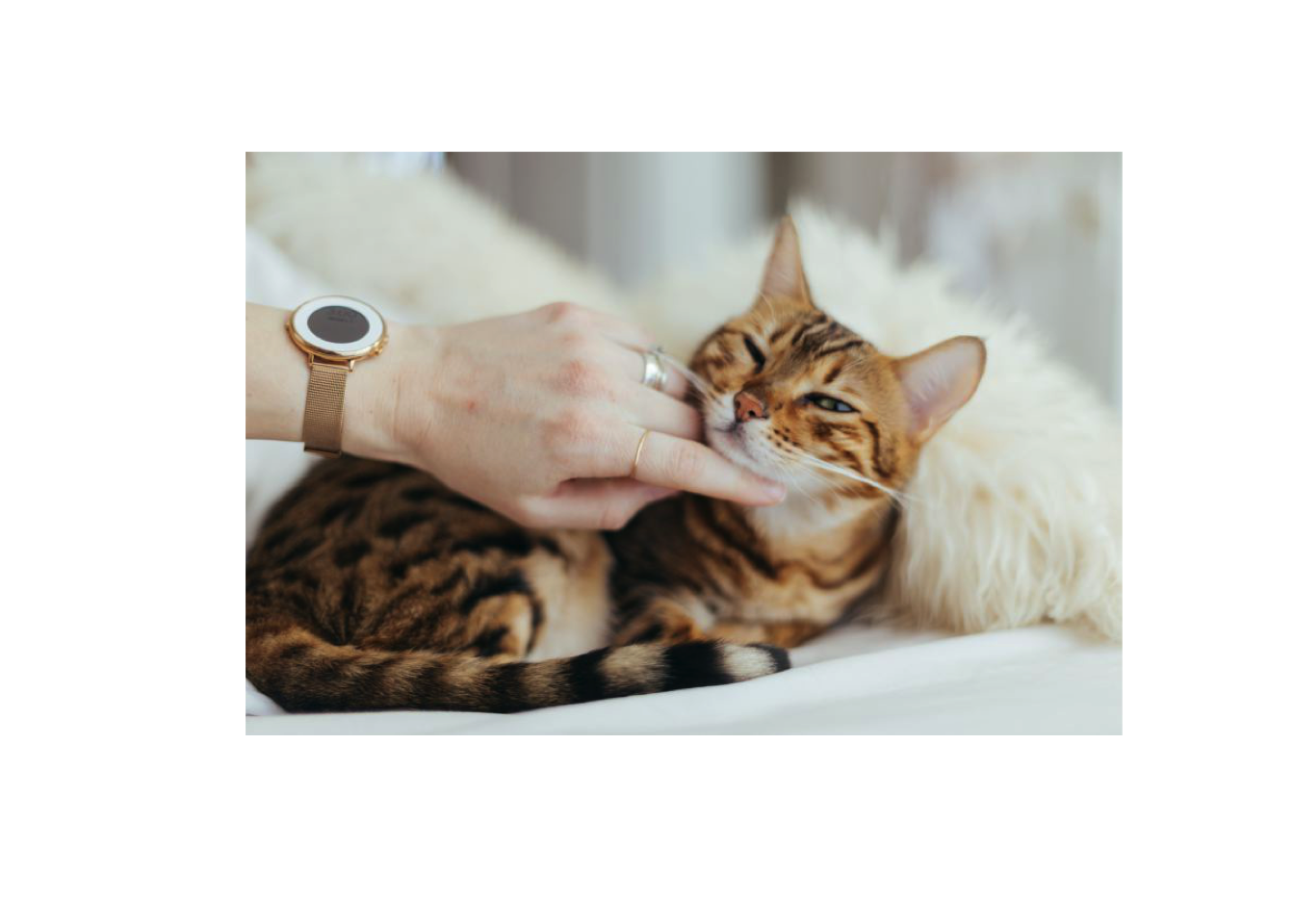

Photo by Paul on Unsplash

Figure 1: Photo by Paul on Unsplash

As with text models the explainer will need to know how to prepare the input data for the model. For keras models this means formatting the image data as tensors. Thankfully keras comes with a lot of tools for reshaping image data:

image_prep <- function(x) {
  arrays <- lapply(x, function(path) {
    img <- image_load(path, target_size = c(224,224))
    x <- image_to_array(img)
    x <- array_reshape(x, c(1, dim(x)))
    x <- imagenet_preprocess_input(x)
  })
  do.call(abind::abind, c(arrays, list(along = 1)))
}
explainer <- lime(img_path, model, image_prep)

We now have an explainer model for understanding how the vgg16 neural network makes its predictions. Before we go along, lets see what the model think of our kitten:

res <- predict(model, image_prep(img_path))
imagenet_decode_predictions(res)

## [[1]]
##   class_name class_description      score
## 1  n02124075      Egyptian_cat 0.48913878
## 2  n02123045             tabby 0.15177219
## 3  n02123159         tiger_cat 0.10270492
## 4  n02127052              lynx 0.02638111
## 5  n03793489             mouse 0.00852214

So, it is pretty sure about the whole cat thing. The reason we need to use imagenet_decode_predictions() is that the output of a keras model is always just a nameless tensor:

dim(res)

## [1]    1 1000

dimnames(res)

## NULL

We are used to classifiers knowing the class labels, but this is not the case for keras. Motivated by this, lime now have a way to define/overwrite the class labels of a model, using the as_classifier() function. Let’s redo our explainer:

model_labels <- readRDS(system.file('extdata', 'imagenet_labels.rds', package = 'lime'))
explainer <- lime(img_path, as_classifier(model, model_labels), image_prep)

There is also an as_regressor() function which tells lime, without a doubt, that the model is a regression model. Most models can be introspected to see which type of model they are, but neural networks doesn’t really care. lime guesses the model type from the activation used in the last layer (linear activation == regression), but if that heuristic fails then as_regressor()/as_classifier() can be used.

We are now ready to poke into the model and find out what makes it think our image is of an Egyptian cat. But… first I’ll have to talk about yet another concept: superpixels (I promise I’ll get to the explanation part in a bit).

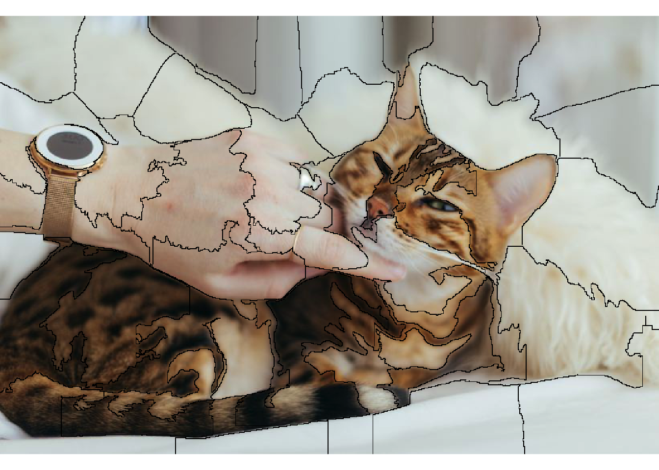
In order to create meaningful permutations of our image (remember, this is the central idea in lime), we have to define how to do so. The permutations needs to be substantial enough to have an impact on the image, but not so much that the model completely fails to recognise the content in every case - further, they should lead to an interpretable result. The concept of superpixels lends itself well to these constraints. In short, a superpixel is a patch of an area with high homogeneity, and superpixel segmentation is a clustering of image pixels into a number of superpixels. By segmenting the image to explain into superpixels we can turn area of contextual similarity on and off during the permutations and find out if that area is important. It is still necessary to experiment a bit as the optimal number of superpixels depend on the content of the image. Remember, we need them to be large enough to have an impact but not so large that the class probability becomes effectively binary. lime comes with a function to assess the superpixel segmentation before beginning the explanation and it is recommended to play with it a bit — with time you’ll likely get a feel for the right values:

# default
plot_superpixels(img_path)

# Changing some settings
plot_superpixels(img_path, n_superpixels = 200, weight = 40)

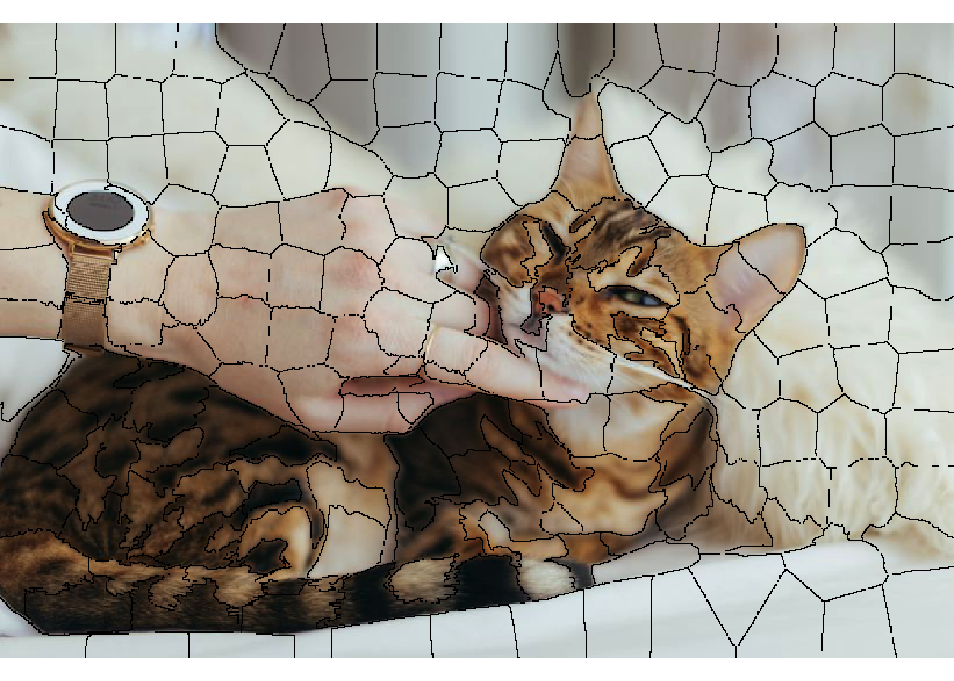
The default is set to a pretty low number of superpixels — if the subject of interest is relatively small it may be necessary to increase the number of superpixels so that the full subject does not end up in one, or a few superpixels. The weight parameter will allow you to make the segments more compact by weighting spatial distance higher than colour distance. For this example we’ll stick with the defaults.

Be aware that explaining image models is much heavier than tabular or text data. In effect it will create 1000 new images per explanation (default permutation size for images) and run these through the model. As image classification models are often quite heavy, this will result in computation time measured in minutes. The permutation is batched (default to 10 permutations per batch), so you should not be afraid of running out of RAM or hard-drive space.

explanation <- explain(img_path, explainer, n_labels = 2, n_features = 20)

The output of an image explanation is a data frame of the same format as that from tabular and text data. Each feature will be a superpixel and the pixel range of the superpixel will be used as its description. Usually the explanation will only make sense in the context of the image itself, so the new version of lime also comes with a plot_image_explanation() function to do just that. Let’s see what our explanation have to tell us:

plot_image_explanation(explanation)

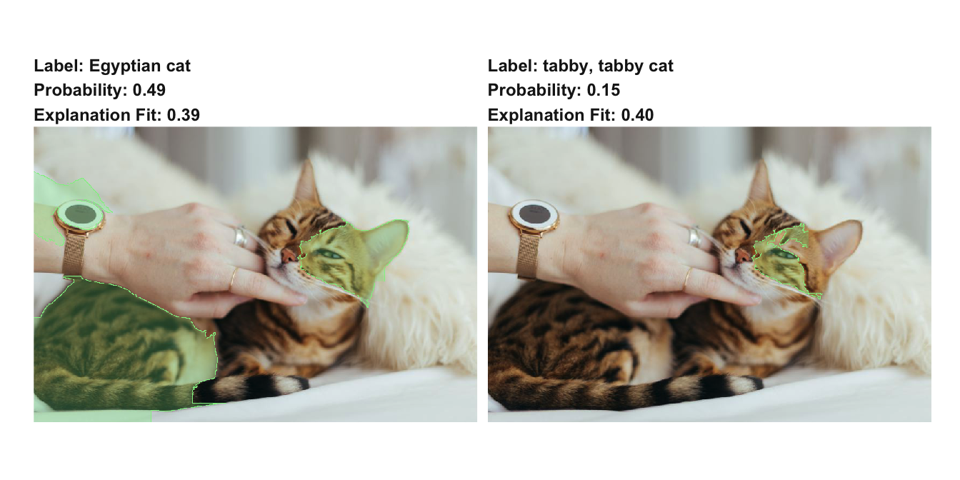
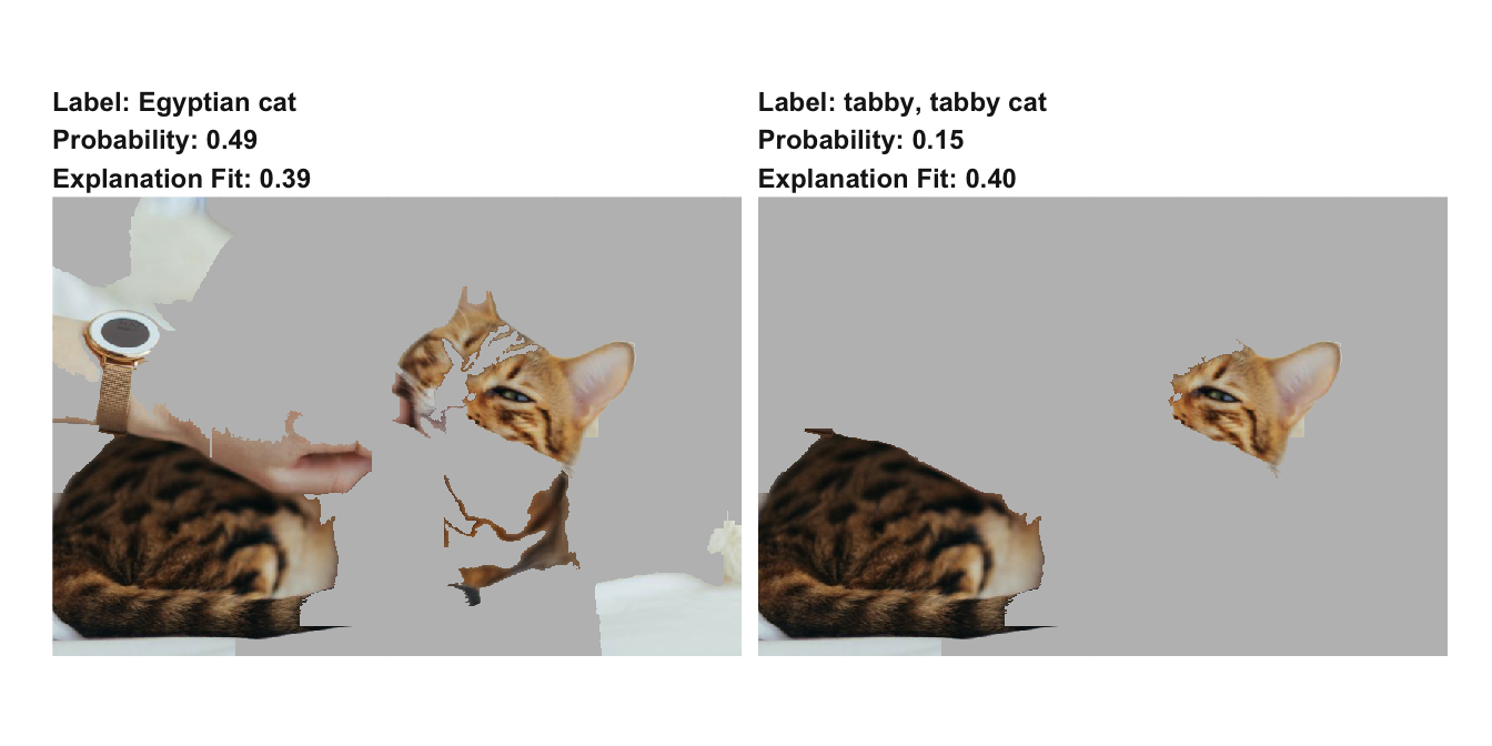
We can see that the model, for both the major predicted classes, focuses on the cat, which is nice since they are both different cat breeds. The plot function got a few different functions to help you tweak the visual, and it filters low scoring superpixels away by default. An alternative view that puts more focus on the relevant superpixels, but removes the context can be seen by using display = ‘block’:

plot_image_explanation(explanation, display = 'block', threshold = 0.01)

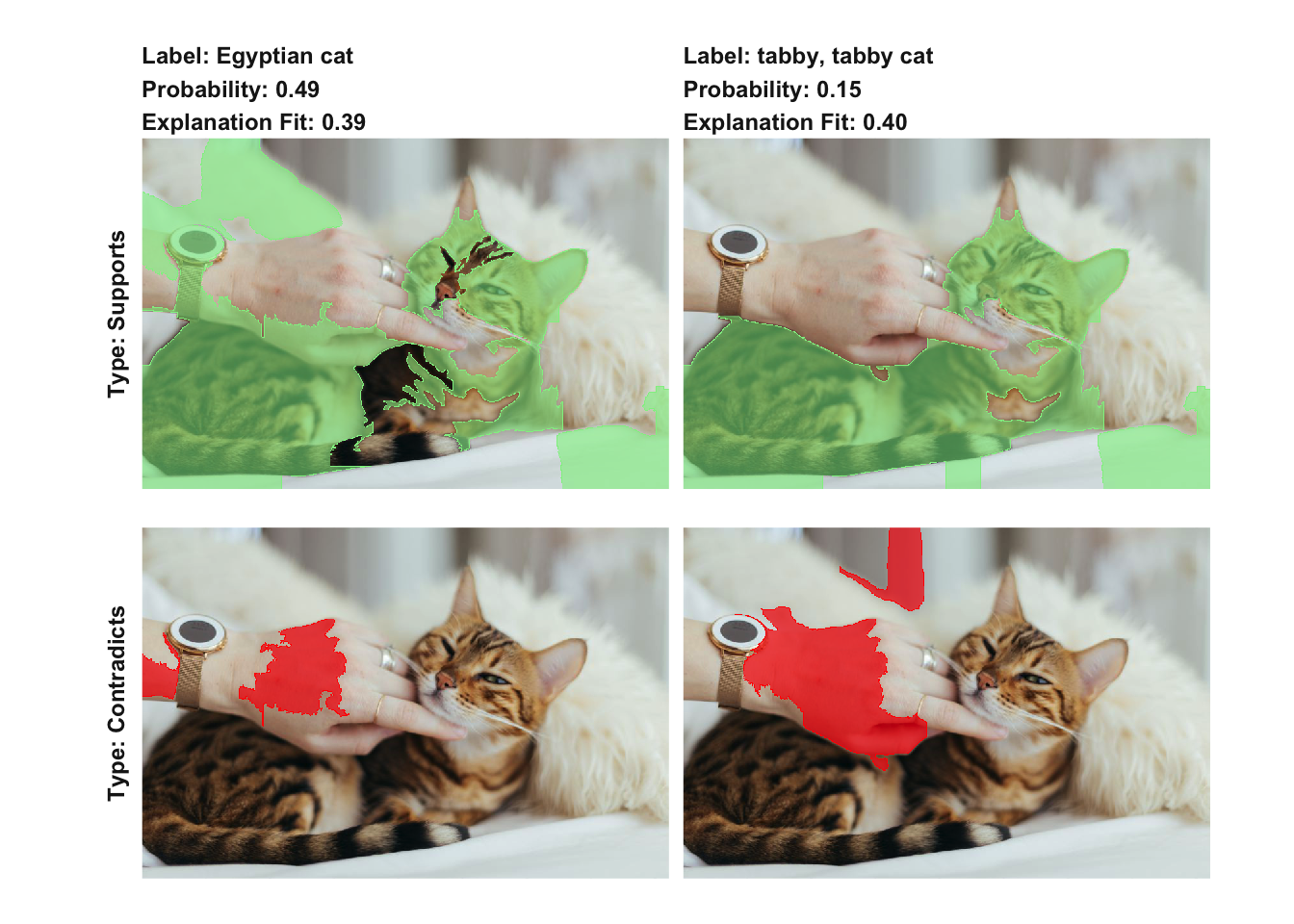
While not as common with image explanations it is also possible to look at the areas of an image that contradicts the class:

plot_image_explanation(explanation, threshold = 0, show_negative = TRUE, fill_alpha = 0.6)

As each explanation takes longer time to create and needs to be tweaked on a per-image basis, image explanations are not something that you’ll create in large batches as you might do with tabular and text data. Still, a few explanations might allow you to understand your model better and be used for communicating the workings of your model. Further, as the time-limiting factor in image explanations are the image classifier and not lime itself, it is bound to improve as image classifiers becomes more performant.

Grab back

Apart from keras and image support, a slew of other features and improvements have been added. Here’s a quick overview:

All explanation plots now include the fit of the ridge regression used to make the explanation. This makes it easy to assess how good the assumptions about local linearity are kept.
When explaining tabular data the default distance measure is now ‘gower’ from the gower package. gower makes it possible to measure distances between heterogeneous data without converting all features to numeric and experimenting with different exponential kernels.
When explaining tabular data numerical features will no longer be sampled from a normal distribution during permutations, but from a kernel density defined by the training data. This should ensure that the permutations are more representative of the expected input.

Wrapping up

This release represents an important milestone for lime in R. With the addition of image explanations the lime package is now on par or above its Python relative, feature-wise. Further development will focus on improving the performance of the model, e.g. by adding parallelisation or improving the local model definition, as well as exploring alternative explanation types such as anchor.

Happy Explaining!